# Libraries
library(tidyverse)

# Importing eshop_revenues
eshop_revenues <- read_csv("https://raw.githubusercontent.com/Datakortex/Datasets/refs/heads/main/eshop_revenues.csv")Multiple Linear Regression and Statistical Inference
Introduction
Multiple linear regression is a natural extension of simple linear regression. While simple linear regression models the relationship between one independent variable and one dependent variable, multiple linear regression allows us to include two or more independent variables in our model. This enables us to better explain the variation in the outcome by considering multiple factors at once.
Simple linear regression can be quite limited—especially when we consider assumptions such as the zero conditional mean. In real-world data, it’s often unrealistic to believe that all omitted factors are uncorrelated with the single independent variable. By including more relevant variables in the model, we reduce the risk of omitted variable bias and get closer to estimating causal relationships. This is where the idea of ceteris paribus—“all else equal”—becomes important. multiple linear regression allows us to isolate the effect of one variable on the dependent variable while holding others constant.
Including more independent variables also means we now estimate more coefficients. In this chapter, we will explore how to derive these OLS estimates in the multiple regression context, how to interpret them, and how the key assumptions change or extend from the simple regression case. We will also discuss statistical inference in multiple regression, including hypothesis testing for individual coefficients and groups of coefficients, and how to assess the overall significance of a model. Finally, we will examine potential pitfalls, such as multicollinearity, and highlight the continued importance of careful model specification.
From Simple Linear Regression to Multiple Linear Regression
To begin, let’s reload our R environment by importing the tidyverse package and loading our dataset eshop_revenues:
A multiple linear regression model takes the following form:
\[y = \beta_{0} + \beta_{1}x_{1} + \beta_{2}x_{2} + u\]
In this model, we still have one dependent variable, \(y\), and an error term, \(u\), just like in simple linear regression. The difference is that we now include two independent variables, \(x_1\) and \(x_2\), each with its own coefficient, \(\beta_1\) and \(\beta_2\). These coefficients represent the effect of each independent variable on the dependent variable, holding the other variable fixed.
This is what allows us to make ceteris paribus interpretations. That is, we can isolate the effect of one variable while keeping all others fixed. For instance, suppose \(y\) represents Revenue, \(x_1\) is Ad_Spend, and \(x_2\) is a Product_Quality_Score. Then the multiple regression model is:
\[\hat{y} = \hat{\beta}_{0} + \hat{\beta}_{1} x_{1} + \hat{\beta}_{2} x_{2}\]
This model allows us to interpret the coefficients as follows:
If \(\hat{\beta}_1 = 30\), then a one-unit increase in \(x_1\) (
Ad_Spend) leads to a 30-unit increase in \(y\) (Revenue), holding \(x_2\) (Product_Quality_Score) constant:\[\Delta{y} = 30 \cdot \Delta{x}_{1}, \ \text{when} \ \Delta{x}_{2} = 0\]
If \(\hat{\beta}_2 = 0.5\), then a one-unit increase in \(x_2\) (
Product_Quality_Score) leads to a 0.5-unit increase in \(y\) (Revenue), holding \(x_1\) (Ad_Spend) constant:\[\Delta{y} = 0.5 \cdot \Delta{x}_{2}, \ \text{when} \ \Delta{x}_{1} = 0\]
These expressions highlight how we can interpret the coefficients independently of each other by isolating the effect of one variable while holding the others fixed. This is the essence of ceteris paribus reasoning in multiple regression.
Like in the simple linear regression case, there is a Population Regression Function that we aim to estimate. However, in practice, we do not know the true values of the coefficients \(\beta_{0}, \beta_{1}, \beta_{2}, \dots, \beta_{k}\). Instead, we use data to estimate them through the Ordinary Least Squares (OLS) method, obtaining the estimates \(\hat{\beta}_{0}, \hat{\beta}_{1}, \hat{\beta}_{2}, \dots, \hat{\beta}_{k}\).
We can include multiple independent variables in the model, allowing us to control for various factors that may influence the dependent variable. That said, as we will discuss later, there are practical and statistical limits to how many variables we can include. In general, a multiple linear regression model with \(k\) independent variables can be written as:
\[y = \beta_{0} + \beta_{1} x_{1} + \beta_{2} x_{2} + ... + \beta_{k} x_{k} + u\]
Visualizing the Linear Regression Line
In multiple linear regression, visualizing the results is generally impossible beyond three dimensions. However, when we have only two independent variables, we can still create meaningful visualizations.
In the plot below, Ad_Spend is on the x-axis and Revenue is on the y-axis. The blue line represents the regression line from a simple linear regression of Revenue on Ad_Spend only. The red line, on the other hand, represents the fitted values from the multiple linear regression where we regress Revenue on both Ad_Spend and Product_Quality_Score. To show the red line in two dimensions, we hold Product_Quality_Score fixed at its mean value. This allows us to isolate the effect of Ad_Spend while controlling for the quality score.
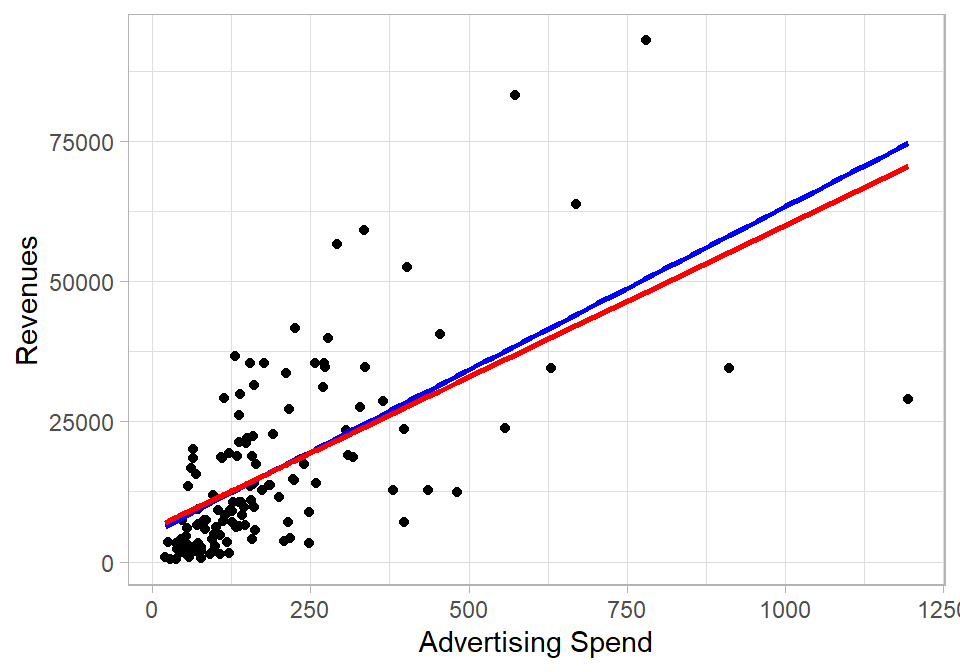
The blue line is actually the best fit in this two-dimensional plot, but it ignores the variation explained by Product_Quality_Score. The red line reflects the adjusted slope of Ad_Spend when we control for the other variable in the model. This shift in the slope happens because the coefficient \(\hat{\beta}_1\) changes when we account for the second variable, capturing the effect of Ad_Spend ceteris paribus.
To better understand how the multiple regression works in three dimensions, we can visualize the regression plane. In the next plot, we display a 3D surface that shows how Revenue changes with both Ad_Spend and Product_Quality_Score. Each point represents an observation, and the red plane is the best linear fit across both predictors:
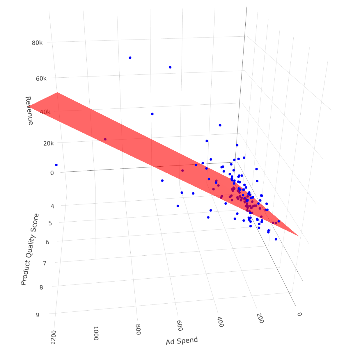
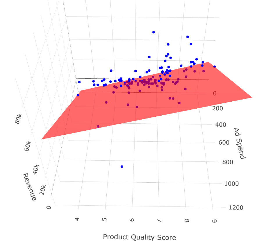
These 3D visualizations provide a more complete but more complicated picture of the regression model, showing how both predictors simultaneously influence the dependent variable. Specifically, the second plot shows when both predictor increase, the expected value of the dependent variable also increases. Additionally, for a fixed level of Product_Quality_Score (e.g., a value of 8), the higher the Ad_spend, the higher the expected value of Revenue; this is exactly what we mean by ceteris paribus.
Deriving Coefficients with OLS
To derive the OLS coefficients in multiple linear regression, we once again rely on the zero conditional mean assumption:
\[E(u | x_{1}, x_{2}, ... x_{k}) = E(u | \mathbf{X}) = 0\]
Here, \(\mathbf{X}\) is a matrix containing all the independent variables. A helpful way to think about this is that \(\mathbf{X}\) is just the data frame of the dataset with only the independent variables.
From the zero conditional mean assumption, the error term is unrelated to any of the independent variables in the model. It implies that each independent variable is uncorrelated with the error term:
\[Cov(u, x_{1}) = 0, \ \ Cov(u, x_{2}) = 0, \ \ ..., \ \ Cov(u, x_{k}) = 0\]
Or, in summation form:
\[\sum^n_{i = 1} x_{ij} u_{i} = 0\]
where \(j = 0, 1, 2, ..., k\) and \(x_{i0}\) represents the intercept.
Now, recall the regression model:
\[y_{i} = \beta_0 + \beta_{1} x_{i1} + \beta_{2} x_{i2} + ... + \beta_{k} x_{ik} + u_{i}\]
Solving for \(u_{i}\), we have:
\[u_{i} = y_{i} - \beta_{0} - \beta_{1} x_{i1} - \beta_{2} x_{i2} - ... - \beta_{k} x_{ik}\]
Here, \(u_{i}\) represents the unobserved error term, which we cannot directly observe. To estimate the coefficients using OLS, we work with the residuals \(\hat{u}_i\) which measure the difference between the observed values and the fitted values from the regression:
\[\hat{u}_{i} = y_{i} - \hat{\beta}_{0} - \hat{\beta}_{1} x_{i1} - \hat{\beta}_{2} x_{i2} - ... - \hat{\beta}_{k} x_{ik}\]
Plugging this into our covariance condition gives us a system of \(k+1\) normal equations:
- For the intercept (where \(x_{i0} = 1\)):
\[\sum^n_{i = 1} \left ( y_{i} - \hat{\beta}_{0} - \hat{\beta}_{1} x_{i1} - \hat{\beta}_{2} x_{i2} - ... - \hat{\beta}_{k} x_{ik} \right ) = 0\]
For each independent variable:
\[\sum^n_{i = 1} x_{ij} \left ( y_{i} - \hat{\beta}_{0} - \hat{\beta}_{1} x_{i1} - \hat{\beta}_{2} x_{i2} - ... - \hat{\beta}_{k} x_{ik} \right ) = 0\]
In expanded form, the system of equations becomes:
\[\sum^n_{i = 1} \left ( y_{i} - \hat{\beta}_{0} - \hat{\beta}_{1} x_{i1} - \hat{\beta}_{2} x_{i2} - ... - \hat{\beta}_{k} x_{ik} \right ) = 0\]
\[\sum^n_{i = 1} x_{i1} \left ( y_{i} - \hat{\beta}_{0} - \hat{\beta}_{1} x_{i1} - \hat{\beta}_{2} x_{i2} - ... - \hat{\beta}_{k} x_{ik} \right ) = 0\]
\[\sum^n_{i = 1} x_{i2} \left ( y_{i} - \hat{\beta}_{0} - \hat{\beta}_{1} x_{i1} - \hat{\beta}_{2} x_{i2} - ... - \hat{\beta}_{k} x_{ik} \right ) = 0\]
\[...\]
\[\sum^n_{i = 1} x_{ik} \left ( y_{i} - \hat{\beta}_{0} - \hat{\beta}_{1} x_{i1} - \hat{\beta}_{2} x_{i2} - ... - \hat{\beta}_{k} x_{ik} \right ) = 0\]
Solving this system gives the OLS estimates for the coefficients. While the solution involves linear algebra or multivariable calculus, we usually let software like R handle the math for us. It is crucial to note, though, that the number of restrictions we get is directly related to the number of independent variables we include in the model. Each variable adds one equation (or restriction) through the zero conditional mean assumption. However, if we include more variables (columns) than data points (rows), the system becomes unsolvable—the matrix of independent variables loses full rank, and OLS cannot compute unique coefficient estimates. Intuitively, this means we are trying to estimate more unknowns than we have information to determine them: there simply isn’t enough data to pin down a unique solution.
The key point is the logic: the coefficients are chosen so that the residuals are uncorrelated with all the independent variables. In other words, once we’ve accounted for the predictors in the model, what’s left (the error) shouldn’t be related to any of them (Montgomery, Peck & Vining, 2021; Greene, 2018).
So, while the multiple regression case involves more equations, the underlying principle is exactly the same as in simple linear regression.
Calculating in R and Interpreting the Results
To fit a multiple linear regression model, we again use the lm() function with the tilde (~) to separate the dependent variable from the independent variables. To include more than one predictor, we simply add them using the + sign. As with simple linear regression, the object created by the lm() function stores much more than just the coefficients, such as the fitted (predicted) values and the residuals).
Let’s create a linear regression model using the dataset we imported:
# Fitting a linear regression model
lm_model <- lm(Revenue ~ Ad_Spend + Product_Quality_Score, data = eshop_revenues)

# Printing coefficients
print(lm_model)
Call:
lm(formula = Revenue ~ Ad_Spend + Product_Quality_Score, data = eshop_revenues)

Coefficients:
          (Intercept)               Ad_Spend
            -29861.84                  54.11
Product_Quality_Score
              5427.83
This output includes the intercept as well as the coefficients for the variables Ad_Spend and Product_Quality_Score. Based on this output, the estimated regression equation is:
\[\widehat{\text{Revenue}}_{i} = -29861.84 + 54.11 \text{AdSpend}_{i} + 5427.83\text{ProductQualityScore}_{i}\]
The interpretation of the estimated coefficients is as follows:
\(\hat{\beta}_0 = -29,861.84\): This is the expected revenue when both
Ad_SpendandProduct_Quality_Scoreare equal to zero. In this context, that interpretation doesn’t make much sense as zero advertising and zero product quality are not realistic business scenarios, and revenue can’t reasonably be negative. Still, this value is part of the mathematical solution that minimizes the sum of squared residuals. The intercept ensures the regression plane is positioned optimally to best fit the data points overall. In many cases, especially when zero values of the independent variables fall outside the range of the observed data, the intercept has no meaningful real-world interpretation, but it is still necessary for the accuracy of the model. We should not ignore it in the regression equation, but we can avoid attaching practical meaning to it when it’s clearly unrealistic.\(\hat{\beta}_1 = 54.11\): This tells us that when
Ad_Spendincreases by 1 unit,Revenueis expected to increase by 54.11 units holdingProduct_Quality_Scorefixed. When we interpret coefficients in multiple regression, we always do so holding all other variables fixed.\(\hat{\beta}_2 = 5,427.83\): Similarly, a one-unit increase in
Product_Quality_Scoreis associated with an increase of approximately €5,428 inRevenue, holdingAd_Spendfixed.
In Chapter Correlation and Simple Linear Regression, the coefficient for Ad_Spend was different, and we saw this in previous plot when we compared the regression lines with and without Product_Quality_Score. Why did the slope change?
This happens because, in multiple regression, each coefficient captures the partial effect of its variable on the dependent variable, controlling for all other variables in the model. In simple regression, the effect of Ad_Spend also absorbs any indirect effects that are actually due to other omitted variables such as Product_Quality_Score. So when we add more variables, the slope for Ad_Spend may change to account for the presence of this new information.
In this example, these estimated coefficients seem logical. We would expect that increasing the Product_Quality_Score would significantly boost revenues—after all, better products are more likely to attract and retain customers. The same applies to Ad_Spend: higher advertising investment tends to increase awareness and sales, leading to higher revenue. The coefficients also make sense from a magnitude perspective. A one-unit increase in product quality is associated with a substantial increase in revenue, while the effect of advertising spend is also positive but more moderate, reflecting the fact that both product quality and advertising contribute to revenue, albeit in different ways. This alignment between the model output and our real-world expectations gives us more confidence in these regression results.
Statistical Properties
The statistical properties of multiple linear regression are essentially the same as those of simple linear regression. As a reminder, the key properties that hold under the standard OLS assumptions are:
1. Sum of residuals is zero:
The residuals from the regression always sum to zero. This ensures that, on average, the predicted values are not systematically above or below the actual values.
2. Sample covariance between each independent variable and the residuals is zero:
After fitting the model, the residuals are uncorrelated with each of the independent variables. This property follows from the OLS estimation procedure, which minimizes the sum of squared residuals.
3. The regression line passes through the average values of the variables:
The fitted regression line (or plane, in higher dimensions) always passes through the point defined by the mean of the dependent variable and the means of the independent variables.
4. Decomposition of total variation:
The total variation in the dependent variable (Total Sum of Squares, TSS) can be decomposed into two parts: the explained variation (Explained Sum of Squares, ESS) and the unexplained variation (Residual Sum of Squares, RSS). That is:
\[\text{TSS} = \text{ESS} + \text{RSS}\]
5. Goodness-of-fit:
R-squared (\(R^2\)) measures the proportion of the total variation in the dependent variable that is explained by the independent variables. While a higher \(R^2\) suggests a better fit, it has important limitations.
One key issue is that \(R^2\) never decreases when new variables are added to the model, even if those variables are completely unrelated to the dependent variable. This happens because both ESS and TSS either increase or stay the same, which mechanically inflates or preserves the value of \(R^2\).
This means \(R^2\) can be misleading when used to judge model quality or compare models with different numbers of predictors. A model might appear to fit better simply because it has more variables, not because those variables are useful. Another problem is that \(R^2\) is a biased estimate of model fit, especially in small samples.
To address the limitations of \(R^2\), especially its tendency to increase mechanically as more variables are added to the model, we often use the adjusted R-squared (\(\bar{R}^2\)). This version of the statistic introduces a correction for the number of predictors by accounting for degrees of freedom. Specifically, it replaces the raw sums of squares (RSS and TSS) in the \(R^2\) formula with their mean squares:
\[\bar{R}^2 = 1 - \frac{\text{RSS} / (n - k - 1)}{\text{TSS} / (n - 1)}\]
Here, \(n\) is the number of observations, and \(k\) is the number of independent variables (excluding the intercept). This adjustment means that \(\bar{R}^2\) can decrease if the added variables do not improve the model enough to justify the loss of degrees of freedom. In fact, if the new predictors are irrelevant, \(\bar{R}^2\) may even become negative. An equivalent and useful alternative expression is:
\[\bar{R}^2 = 1 - (1 - R^2) \cdot \frac{n - 1}{n - k - 1}\]
Notice the term \(\frac{n - 1}{n - k - 1}\). As we add more independent variables to the model, \(k\) increases, which makes the denominator smaller. This, in turn, makes the entire fraction larger, increasing the amount we subtract from 1. As a result, even if \(R^2\) stays the same or increases only slightly, the \(\bar{R}^2\) can decrease, because the model is being penalized for using more predictors. This ensures that only variables that genuinely improve the fit of the model (beyond what could happen by chance) will lead to a higher \(\bar{R}^2\).
This makes it clear that \(\bar{R}^2\) imposes a penalty on models with many predictors, providing a more reliable measure of goodness-of-fit when comparing models with different numbers of variables.
Assumptions
The assumptions required for multiple linear regression are similar to those we discussed in the context of simple linear regression. These assumptions are essential for the Ordinary Least Squares (OLS) estimates to be unbiased and efficient (i.e., have the smallest variance among all linear unbiased estimators) (Wooldridge, 2022). Here is a summary of the key assumptions:
1. Linear in Parameters:
The regression model must be linear in the coefficients (parameters). This means the relationship between the dependent variable and the independent variables can be expressed as:
\[y_i = \beta_{0} + \beta_{1} x_{i1} + \beta_{2} x_{i2} + ... + \beta_{k} x_{ik} + u_{i}\]
2. Random Sampling:
Each observation is randomly and independently drawn, ensuring the data are representative and unbiased.
3. No Perfect Collinearity and Sample Variation in the Independent Variables:
There must be variation in each independent variable, and no independent variable should be a perfect linear combination of the others. If perfect collinearity exists, it’s like including the same information twice, and the model won’t be able to uniquely estimate the coefficients—mathematically, the system of equations has no unique solution.
4. Zero Conditional Mean:
The error term \(u_i\) must have an expected value of zero given any combination of the independent variables:
\[E(u_{i} | x_{i1}, x_{i2}, ..., x_{ik}) = E(u | \mathbf{X}) = 0\]
This assumption implies that there are no omitted variables that are correlated with both the dependent variable and any of the independent variables. While the form of the assumption stays the same as in simple linear regression, in practice it becomes more plausible in the multiple regression setting because we can include more relevant variables that might otherwise be omitted. That said, including the “right” variables is crucial — if relevant variables are left out, or if irrelevant ones are included, the assumption may still fail.
5. Homoskedasticity:
The variance of the error term should be constant across all values of the independent variables:
\[Var(u_{i} | x_{i1}, x_{i2}, ..., x_{ik}) = Var(u | \mathbf{X}) = \sigma^2\]
This means that the spread of the residuals is the same regardless of the values of the predictors. When this assumption is violated (i.e., we have heteroskedasticity), OLS estimates remain unbiased, but the variance and standard errors become unreliable.
If the first four assumptions hold—linearity, random sampling, no perfect collinearity, and zero conditional mean—then the OLS estimator is unbiased, meaning that on average, it correctly estimates the true population coefficients.
If, in addition, the fifth assumption of homoskedasticity also holds, then the OLS estimator is efficient among all linear unbiased estimators. If all these assumptions hold, then Ordinary Least Squares (OLS) is BLUE according to the Gauss-Markov Theorem (Wooldridge, 2022).
Once again, violations of homoskedasticity don’t bias the coefficient estimates—the expected values remain correct—but the estimates become less precise.
Estimator Variance in Multiple Linear Regression
When it comes to the variance of a coefficient of an independent variable, the formula is now different. Each coefficient has its own variance and thus its own standard error:
\[Var(\hat{\beta}_{i}) = \frac{\sigma^2}{\text{SST}_{j} \cdot (1 - R^2_{j})}\]
The two components are familiar to us. A larger \(\sigma^2\) means larger residuals, which implies higher uncertainty in our estimates. The \(\text{SST}_{j}\) is the total variation of the independent variable \(x_{j}\). Just like in simple linear regression, the more variation we have in an independent variable, the more precisely we can estimate its coefficient.
The new element here is the \(R^2_{j}\) in the denominator. This is not the R-squared from our main regression model. Instead, \(R^2_{j}\) refers to the R-squared from a separate regression in which \(x_{j}\) is regressed on all the other independent variables. In this case, \(x_{j}\) becomes the dependent variable, and we assess how well it can be predicted by the remaining independent variables. That’s why we use the subscript \(j\)—it tells us which variable is being “explained” (Montgomery et al., 2021).
This component captures multicollinearity: if \(x_{j}\) is highly correlated with the other independent variables, then \(R^2_{j}\) will be close to 1, and the denominator becomes small, inflating the variance of \(\hat{\beta}_{j}\). This makes our estimates less precise and leads to higher standard errors.
In practice, we do not know the true error variance \(\sigma^2\), since we do not observe the true errors \(u_{i}\). Instead, we estimate it using the residuals \(\hat{u}_{i}\) from our sample. This gives us the residual variance, often denoted as \(\hat{\sigma}^2\), and it serves as our estimate of the population error variance:
\[\sigma^2 = \frac{1}{n - k - 1} \sum^n_{i = 1} \hat{u}^2_{i}\]
Here, \(n\) is the sample size and \(k\) is the number of independent variables. We divide by \(n - k - 1\) to account for the degrees of freedom used in estimating the \(k + 1\) parameters (including the intercept). This correction ensures that our estimate of the variance is unbiased.
Once we have this estimate of the error variance, we plug it into the earlier formula to estimate the variance of a coefficient. The standard error of \(\hat{\beta}_{j}\) is then simply the square root of that estimated variance:
\[SE(\hat{\beta}_{j}) = \sqrt{\frac{\sigma^2}{\text{SST}_{j} \cdot (1 - R^2_{j})}}\]
This standard error tells us how much the estimated coefficient \(\hat{\beta}_{j}\) would vary if we were to draw many different samples from the population and re-estimate the model each time. The larger the standard error, the less precise our estimate is—making it harder to determine if \(\hat{\beta}_{j}\) s statistically different from zero.
Residual Variance and Its Role in Coefficient Precision
To clarify, in a regression model, the residual variance \(\hat{\sigma}^2\) reflects the average squared difference between the observed values of the dependent variable and the values predicted by the model. This is actually the SSR metric. By using the residual variance, we are able to measure the variance of the distribution of the estimated coefficients. Specifically, \(\hat{\sigma}^2\) is used in the denominator of the variance formulas for the coefficient estimates, helping us calculate how much the estimates would vary from sample to sample. In other words, the more spread-out the residuals are, the more uncertainty we have in our coefficient estimates. This is why a higher residual variance leads to larger standard errors and why reducing unexplained variation improves the precision of our model.
Multicollinearity
As noted above, multicollinearity occurs when independent variables are highly correlated. There is a common misconception that when we use OLS, we assume no multicollinearity, something that is not true. There is actually no universal rule about what we need to do when two variables are highly correlated but they both are very important to the dependent variable. For example, suppose we are trying to explain house prices using both house size (m²) and the number of rooms. These two variables are highly correlated because larger houses usually have more rooms. However, both clearly matter for predicting price: size captures overall space, while number of rooms captures layout and usability. Even though they move together, dropping one would risk leaving out a meaningful part of what determines house prices.
Multicollinearity does not violate key assumptions for unbiasedness or efficiency, such as the zero conditional mean or homoskedasticity, but it does introduce practical challenges for both precision and interpretation. When two variables move closely together, the model struggles to determine how much of the variation in the dependent variable is attributable to each one. This inflates the standard errors of the affected coefficients, increasing their uncertainty (Greene, 2018; Montgomery et al., 2021).
Regarding interpretation, we know that adding or removing a variable changes the coefficients of others in the model. When two variables are highly correlated, the estimated coefficients can change dramatically if one is excluded—sometimes even reversing the direction of the effect. This complicates understanding the true impact of each independent variable on the dependent variable.
To see this in practice, let’s fit a multiple linear regression model. This time, we include both Ad_Spend and Website_Visitors as independent variables. First, let’s check the correlation between these two predictors:
# Correlation between Ad_Spend and Website_Visitors
cor(eshop_revenues$Ad_Spend, eshop_revenues$Website_Visitors)
[1] 0.4568004Even though the correlation is not extremely high, it’s strong enough to illustrate the potential issue of multicollinearity. If we regress Revenue only on Ad_Spend, we get a coefficient of 58.17. However, when we include Website_Visitors in the model as well, the results change:
# Fitting a linear regression model
lm_model <- lm(Revenue ~ Ad_Spend + Website_Visitors, data = eshop_revenues)

# Printing coefficients
print(lm_model)
Call:
lm(formula = Revenue ~ Ad_Spend + Website_Visitors, data = eshop_revenues)

Coefficients:
     (Intercept)          Ad_Spend  Website_Visitors
        -9417.34             48.05             14.29
The coefficient for Ad_Spend drops to 48.05. This is a notable change, showing how the inclusion of a correlated predictor can affect the interpretation of coefficients. It suggests that part of the variation in Revenue that was originally attributed to Ad_Spend is now being shared with Website_Visitors. This is a key symptom of multicollinearity: it becomes harder to isolate the unique effect of each variable on the dependent variable.
In extreme cases, where one independent variable is a perfect linear combination of others (perfect multicollinearity), the model cannot be estimated at all—violating the no perfect collinearity assumption—and R or any other statistical software will return an error or omit the problematic variable.
In summary, multicollinearity does not violate assumptions for unbiasedness or efficiency and does not break the model, but it significantly complicates interpretation (Wooldridge, 2022).
The Impact of Adding or Removing Independent Variables
We saw earlier that adding or removing an independent variable can change the coefficient estimates of the other variables. When we have many variables to choose from, several scenarios can arise—each with different implications for the accuracy and precision of our estimates.
Excluding irrelevant predictors:
If a variable has no true effect on the dependent variable and is also uncorrelated with the other predictors, excluding it causes no harm. The model remains correctly specified, the error term is unaffected, and the coefficient estimates of the included variables remain unbiased and efficient. In this case, we enjoy the benefits of a simpler model with no trade-off in accuracy or precision.
Adding irrelevant predictors:
Including a variable that has no relationship with the dependent variable and is uncorrelated with the other predictors does not affect the unbiasedness of the coefficient estimates. However, it introduces a trade-off: the additional variable reduces the degrees of freedom and adds noise to the model. This inflates the standard errors, making the estimates less precise, even though they remain centered around the true values in repeated samples. In short, we maintain unbiasedness but lose precision.
Excluding relevant predictors:
This is a much more serious issue. If we omit a variable that is correlated with the dependent variable and also correlated with one or more included independent variables, then this omitted variable becomes part of the error term \(u\). In this case, the zero conditional mean assumption fails, because the error term is now correlated with the included independent variables. This leads to biased and inconsistent estimates. More specifically, the coefficients of any included variables that are correlated with the omitted variable will generally be biased and inconsistent. Variables that are not correlated with the omitted variable may remain unbiased, although in practice omitted variable bias often affects multiple coefficients simultaneously.
In terms of standard errors, the model may still report them, but they will be misleading because the bias contaminates the interpretation. In this scenario, both the accuracy and the interpretability of the model suffer.
Adding relevant predictors with high correlations:
This is the trickiest scenario. Suppose we include two relevant predictors that are highly correlated with each other. This avoids omitted variable bias and keeps our estimates unbiased, assuming the model is otherwise correctly specified. However, the high correlation introduces multicollinearity, which inflates the standard errors of the affected coefficients.
This inflation makes the estimates less precise, sometimes to the point where even truly important variables appear statistically insignificant. So we face a trade-off: include both and preserve unbiasedness but risk imprecision, or drop one and risk introducing bias.
Controlling for other variables:
One of the main reasons we include additional variables in a regression model is to control for their effects. By doing this, we isolate the relationship between a particular independent variable and the dependent variable, holding all else constant. In other words, we exclude these control variables from the error term and make it more likely that the zero conditional mean assumption holds.
This is a standard practice in empirical research. Even if we are not interested in the coefficients of certain variables, we include them to account for confounding factors that might distort the estimated relationship between the variable of interest and the outcome. In doing so, we improve the credibility of any causal claims we might want to make.
From Estimation to Hypothesis Testing
In linear regression, knowing the expected value and variance of an estimated coefficient is essential for understanding the key properties of unbiasedness and efficiency. However, knowing the expected value and the variance of a sampling distribution of an estimated coefficient, does not say anything about the form of the distribution; it could be normal uniform or even poisson.
This means that the expected value and variance are not sufficient alone for making statistical inference—that is, drawing conclusions about the population from the sample data. Statistical inference relies on theoretical probability distributions to quantify uncertainty and evaluate the likelihood of various hypotheses.
The distribution we use for inference depends on the context. In the case of linear regression, statistical inference typically builds on the sampling distribution of the estimated coefficients, which—under certain assumptions—follows a t-distribution.
In a nutshell, a t-distribution is a distribution that is similar in shape to the standard normal distribution but has heavier tails, reflecting the additional uncertainty from estimating the population variance from a sample. We use it in this context because the true variance of the error terms is unknown and must be estimated from the data, which introduces extra variability—especially in smaller samples—making the t-distribution more appropriate than the normal distribution for inference on the coefficients. As the sample size increases, however, this extra uncertainty diminishes, and the t-distribution becomes nearly indistinguishable from the normal distribution.
Let us now return to the multiple linear regression model. We regress Revenue on Ad_Spend, Product_Quality_Score, and Website_Visitors:
# Fitting a linear regression model
lm_model <- lm(Revenue ~ Ad_Spend +
                 Product_Quality_Score +
                 Website_Visitors,
               data = eshop_revenues)

# Printing coefficients
print(lm_model)
Call:
lm(formula = Revenue ~ Ad_Spend + Product_Quality_Score + Website_Visitors,
    data = eshop_revenues)

Coefficients:
          (Intercept)               Ad_Spend
           -35222.037                 48.888
Product_Quality_Score       Website_Visitors
             5030.115                  7.791
This model provides us with estimated coefficients for each independent variable. Suppose the estimated regression equation is:
\[\widehat{\text{Revenue}} = -35222 + 48.9 \text{AdSpend} + 5030.1 \text{ProductQualityScore} + 7.8 \text{WebsiteVisitors}\]
Now that we have the coefficient estimates, we are equipped to interpret the expected change in revenue associated with each independent variable. But an important question remains: are these effects statistically significant? For example, if the coefficient on Website_Visitors is 0.001, it implies that, holding other variables constant, revenue is expected to increase by only €1 for every 1,000 additional visitors. This effect may be negligible in practice. We need statistical inference to determine whether such an effect is distinguishable from zero in the population, or whether it could simply be the result of random sampling variation.
To make statistical inference, we must formulate a null hypothesis and an alternative hypothesis to guide our inference. In regression analysis, we typically test whether each coefficient is significantly different from zero. For example, the hypotheses for the coefficient on Ad_Spend might be:
\(H_0: \beta_1 = 0\)
\(H_1: \beta_1 \ne 0\)
To evaluate these hypotheses, we conduct a one sample t-test for each coefficient. The formula for the t-statistic is:
\[t = \frac{\hat{\beta}_{i} - \beta_{i}}{SE(\hat{\beta}_{i})}\]
Here, \(\hat{\beta}_{i}\) is the estimated coefficient, \(\beta_{i}\) is the hypothesized value under the null (typically 0), and \(SE(\hat{\beta}_{i})\) is the standard error of the estimate. The standard error is derived from the residual variance of the model and reflects how much the estimate would vary across repeated samples.
Once we have the t-value, we compare it to the t-distribution with the appropriate degrees of freedom to determine whether the observed value is extreme enough to reject the null hypothesis. For instance, assuming a 5% threshold, a t-value of 1 would be considered too close to 0; only the green area is considered to be far enough from 0 to be considered significant. In the plot below, only values falling in the green shaded regions are considered sufficiently far from 0 to be statistically significant. Together, these regions account for 5% of the total area under the distribution, corresponding to the significance level chosen before conducting the test.
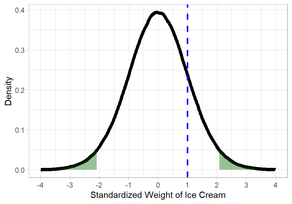
Therefore, the larger the absolute value of the t-statistic, the greater the evidence against the null hypothesis. The formula for the t-statistic also makes intuitive sense: a large estimated coefficient or a small standard error (indicating low uncertainty about the estimate) will produce a larger t-value, placing the statistic farther from 0. Notice that in this example we do not distinguish between positive and negative effects; we are simply testing whether the coefficient differs from 0. Although the hypothesized value can be any number, in practice it is most often 0.
If the difference between the estimated coefficient \(\hat{\beta}_{i}\) and the hypothesized value \(\beta_{i}\) is small with high uncertainty (high standard error), the whole fraction would be close to the center of the t-distribution. Such a case would produce high p-values, indicating that based on data, there is little evidence against the null hypothesis. Consequently, we fail to reject the null hypothesis and conclude that the observed difference could plausibly be explained by random sampling variation alone. The p-value is the probability of observing a result at least as extreme as the one we got, if the null hypothesis is actually correct. This probability is actually illustrated in the plot below:

Notice how the blue shaded area begins at a t-value of 1 on the right-hand side of the distribution. Because this is a two-sided test, we also include the symmetric region on the left-hand side beginning at -1. Together, these two shaded regions represent the p-value: the probability of obtaining a test statistic at least as extreme as the observed value, assuming the null hypothesis is true. In this example, the blue shaded area is larger than the pre-specified significance level of 5%. Therefore, the observed t-statistic is not considered sufficiently extreme, and we fail to reject the null hypothesis. In other words, the data do not provide enough evidence to conclude that the coefficient is statistically significantly different from 0.
Having reviewed the logic behind hypothesis testing, p-values, and the t-distribution, we can now return to our multiple regression model. Fortunately, we do not need to calculate t-statistics or p-values by hand. The coefficients, standard errors, t-values, and their corresponding p-values are all automatically computed when we use the lm() function in R. To access and display them, we use the summary() function on the model object. This summary provides a complete overview of the estimated coefficients, their variability across samples, the results of the hypothesis tests (via the t-values), and the associated p-values that indicate whether each coefficient is statistically significant:
# Printing detailed regression output
lm_model %>% summary()
Call:
lm(formula = Revenue ~ Ad_Spend + Product_Quality_Score + Website_Visitors,
    data = eshop_revenues)

Residuals:
   Min     1Q Median     3Q    Max
-37767  -6250   -745   3936  46169

Coefficients:
                        Estimate Std. Error t value Pr(>|t|)
(Intercept)           -35222.037   5749.350  -6.126 1.06e-08 ***
Ad_Spend                  48.888      5.914   8.267 1.64e-13 ***
Product_Quality_Score   5030.115    784.281   6.414 2.60e-09 ***
Website_Visitors           7.791      3.944   1.975   0.0504 .
---
Signif. codes:  0 '***' 0.001 '**' 0.01 '*' 0.05 '.' 0.1 ' ' 1

Residual standard error: 10510 on 126 degrees of freedom
Multiple R-squared:  0.5849,    Adjusted R-squared:  0.575
F-statistic: 59.17 on 3 and 126 DF,  p-value: < 2.2e-16
This output contains several important elements that allow us to perform statistical inference.
Let us walk through the key parts:
Call: The first line displays the formula used to specify the model. This helps verify that we regressed the correct dependent variable on the appropriate predictors.Residuals: This section summarizes the distribution of the residuals—i.e., the differences between the observed and predicted values of the dependent variable. It reports five summary statistics: the minimum, 1st quartile, median, 3rd quartile, and maximum. Ideally, the residuals should be symmetrically distributed around zero, which would support the assumption of zero-mean errors.Coefficients: This is the core table for inference. Each row corresponds to a model parameter (intercept or slope), and each column provides important information.Estimate: The estimated value of the coefficient \(\hat{\beta}_{i}\).Std. Error: The standard error of the estimate, reflecting its variability across repeated samples.t value: The test statistic used to assess whether a coefficient is significantly different from zero. It is calculated as:\[t = \frac{\hat{\beta}_{i} - \beta_{i}}{SE(\hat{\beta}_{i})} = \frac{\hat{\beta}_{i}}{SE(\hat{\beta}_{i})}\]
where the second equality follows from the null hypothesis \(H_0: \beta_i = 0\). The larger the absolute value of the t-statistic, the stronger the evidence against the null hypothesis.
Pr(>|t|): The p-value associated with the t-test. A small p-value (typically below 0.05) provides evidence against the null hypothesis, suggesting that the coefficient is statistically significant.
The table may also include symbols such as * or ** to indicate significance levels, often based on conventional thresholds (e.g., 0.1, 0.05, 0.01). These visual cues help quickly identify which predictors are statistically significant.
Residual standard error: This is an estimate of the standard deviation ( \(\sqrt{\sigma^2}\) )of the residuals.
Degrees of freedom: This tells us how many observations and predictors were used, which determines the shape of the t-distribution used in the hypothesis tests.
R-squared and Adjusted R-squared: These values summarize how well the model explains the variability in the dependent variable. R-squared gives the proportion of variance explained by the model, while the adjusted version accounts for the number of predictors, penalizing unnecessary complexity.
The F-statistic and its p-value measure the overall significance of the model, that is, whether all regression coefficients are jointly significantly different from 0.
Regarding our example output, the p-values for almost all coefficients are statistically significant at the 5% significance level, indicating that these predictors have meaningful associations with the dependent variable. One borderline case is the coefficient for Website_Visitors, which has a p-value of 0.0504 which slightly above the conventional 5% threshold. While this technically does not meet the cutoff for significance, it is extremely close, and such small differences are often considered with caution and interpreted in context rather than rigidly.
The R-squared and Adjusted R-squared values are 58.49% and 57.50%, respectively. The fact that these two values are close suggests that the model does not include unnecessary predictors. The Adjusted R-squared penalizes the inclusion of additional variables that do not improve the model, so when it remains close to the R-squared, it provides reassurance that each variable contributes meaningfully to explaining the variation in the dependent variable.
Assumption of Statistical Inference
As stated earlier, knowing the expected value and variance of an estimated coefficient is helpful for understanding unbiasedness and efficiency. However, it is not sufficient for making statistical inference. To conduct hypothesis tests, such as the t-test, we rely on theoretical distributions. This introduces one additional assumption required for inference in the classical linear regression model: the normality assumption, which states that the error terms in the regression model are normally distributed with a mean of zero and constant variance. Mathematically, this is written as:
\[u \sim N(0, \sigma^2)\]
We have already assumed that the error terms have an expected value of zero (i.e., they are centered around zero), and that they all share the same constant variance, \(\sigma^2\). The normality assumption adds that the shape of the distribution is also known: it is bell-shaped, symmetric, and follows the normal (Gaussian) distribution.
This assumption carries over to the distribution of the dependent variable \(y\) conditional on the values of the independent variables \(\mathbf{X}\). In other words:
\[y | \mathbf{X} \sim N(\beta_0 + \beta_1x_1 + \beta_2 x_2 + ... + \beta_k x_k, \sigma^2)\]
This means that for any fixed point in the multidimensional space of the independent variables, the value of \(y\) is normally distributed around its conditional mean. That is, holding the independent variables fixed, \(y\) behaves like a normal random variable.
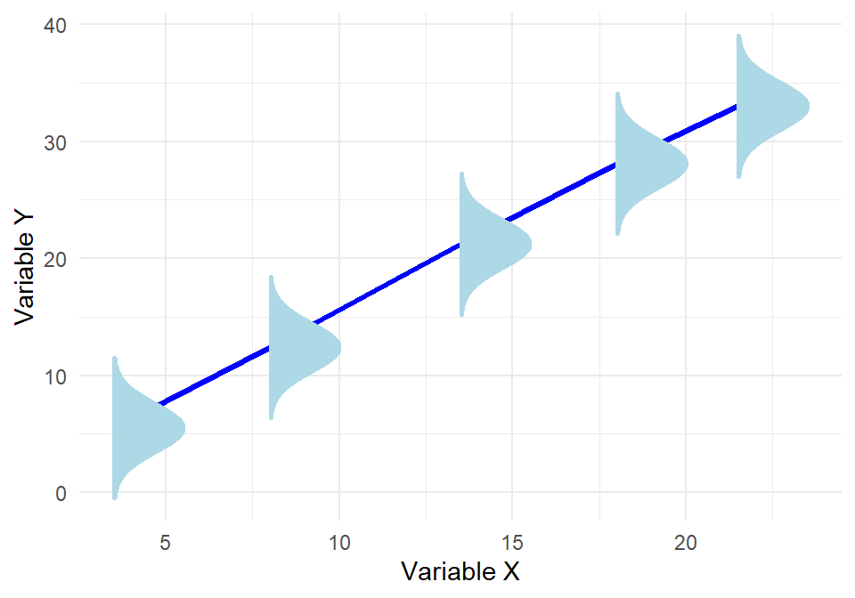
The plot below illustrates a key assumption of linear regression: that the response variable \(y\) follows a normal distribution around the regression line at every value of \(x\). At several points along the line, we’ve visualized this by drawing normal distribution “tunnels”, each centered at the predicted value of \(y\) for a given \(x\). This highlights the normality assumption of the errors—that the variability in \(y\) at each level of \(x\) is random and normally distributed. If this assumption holds, and the relationship between \(x\) and \(y\) is truly linear, then the red regression line represents the best possible linear estimate of the expected value of \(y\) given \(x\). In other words, under these conditions, there is no better straight line we could draw to capture the average behavior of \(y\) across values of \(x\).
Because the OLS estimates are linear combinations of the dependent variable \(y\), and \(y\) is normally distributed, it follows that the estimated coefficients themselves are also normally distributed:
\[\hat{\beta}_j \sim N(\beta_j, Var(\hat{\beta}_j))\]
More generally, any linear combination of the estimated coefficients, such as \(c_1 \hat{\beta}_1 + c_2 \hat{\beta}_2\), is also normally distributed. This property allows us to construct confidence intervals and conduct hypothesis tests on individual coefficients as well as combinations of them.
An example of where normality would not hold can be viewed in the plot below:
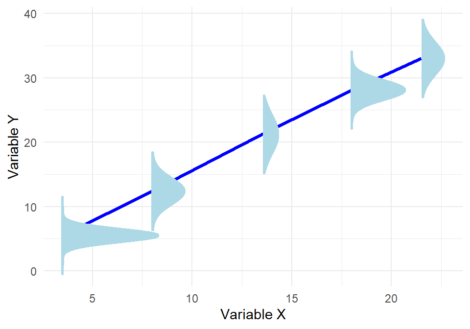
Even though the regression line fits the data very well, the spread of the points around the line is not the same everywhere—some points are very close to the line, while others are much more spread out. If we ask, “Is the estimated slope statistically significantly different from 0?”, the answer can depend on which part of the x-axis we are looking at. In other words, we are no longer fully confident about whether the estimated slope of the regression line is truly different from 0.
The plot above also illustrates that it is possible to have normal distributions with different variances around the regression line. In this case, the errors are still centered around zero at each value of x, but the spread of the distribution changes depending on x. This is an example of heteroskedasticity with conditional normality. In such a setting, the normality assumption can still hold locally, but the constant variance assumption is violated, meaning that the precision of our estimates differs across values of the independent variable.
Thus, for standard OLS inference (including hypothesis testing and confidence intervals) to be valid, we rely on the five classical assumptions discussed in earlier chapters:
Linearity in parameters
Random and independent sampling
Sample variation and no perfect multicollinearity
Zero conditional mean of errors
Homoskedasticity (constant error variance)
By adding normality of the error terms, we now have a sixth assumption. Together, these six assumptions define what is known as the Classical Linear Model (CLM). Under these assumptions, OLS estimators in cross-sectional data are not only BLUE (Best Linear Unbiased Estimators, as stated by the Gauss-Markov theorem), but also normally distributed, allowing us to perform valid statistical inference using t- and F-tests (Wooldridge, 2022).
Surprisingly, even if the normality assumption is violated, statistical inference may still be valid when the sample size is sufficiently large. This is due to the Central Limit Theorem (CLT). The CLT states that, under certain regularity conditions, the distribution of the sample mean (and more generally, linear estimators such as OLS) approaches a normal distribution as the sample size increases. This means that, in large samples, the estimated coefficients will still be approximately normally distributed, even if the original error terms are not. As a result, t-tests and confidence intervals based on the normal distribution become asymptotically valid (Wooldridge, 2022).
The term asymptotically refers to what happens as the sample size tends toward infinity. In other words, asymptotic properties describe the behavior of estimators when we imagine having more and more data. An estimator is said to be asymptotically normal if its distribution becomes closer to the normal distribution as the sample size increases. Similarly, a test is asymptotically valid if its conclusions (e.g., rejecting or not rejecting the null hypothesis) become increasingly accurate and reliable with more data.
It is important to note that asymptotic results are not exact in finite samples. They are approximations that improve with larger sample sizes. Therefore, in small datasets, we still prefer to assume normality explicitly if we want to use t-tests or construct confidence intervals.
The concept of asymptotic validity may not seem practical and in fact it isn’t; it is primarily theoretical. It helps us understand the long-run behavior of estimators and statistical tests under general conditions. In practice, we never observe an infinite sample—so these results guide our expectations and justify the use of certain methods in large samples, rather than serving as a guarantee in every case.
The bottom line is that normality is crucial for making exact inferences in small samples. It allows us to use the t-distribution to construct confidence intervals and perform hypothesis testing on regression coefficients. However, in large samples, even if the error terms are not perfectly normal, the Central Limit Theorem helps ensure that our estimates and statistical tests remain approximately valid. In this way, normality is a helpful but not always essential assumption—its importance depends on the sample size.
Recap
In this chapter, we explored how the transition from simple to multiple linear regression brings both new opportunities and new challenges. While the goal remains the same—understanding relationships between variables—adding more predictors allows us to have better control over our estimators and better isolate effects. At the same time, it introduces complexities such as multicollinearity and changes in how we interpret coefficients.
We discussed how assumptions like zero conditional mean and homoskedasticity still apply, but new concerns emerge around model specification and variable inclusion. We examined how adding or excluding variables can affect bias, variance, and standard errors, and how residual variance plays a key role in estimating the precision of our coefficients. We also introduced statistical inference in the multiple regression setting, including hypothesis testing, t-statistics, p-values, confidence intervals, and the interpretation of coefficient significance. Ultimately, multiple regression offers greater flexibility but demands more care in how we build, evaluate, and interpret models.